
Butterworth Filter Design in MATLAB: Low-Pass and High-Pass
Advertisement
This article presents MATLAB code for designing Butterworth Low-Pass and High-Pass filters.
Butterworth Low-Pass Filter MATLAB Code
%Butterworth Low Pass Filter
clc;
close all;
clear all;
format long;
rp=input('enter the passband ripple:(default:0.15)');
rs=input('enter the stopband ripple:(default:60)');
wp=input('enter the passband frequency:(default:1500)');
ws=input('enter the stopband frequency:(default:3000)');
fs=input('enter the sampling frequency:(default:7000)');
w1=2*wp/fs;
w2=2*ws/fs;
[n,wn]=buttord(w1,w2,rp,rs,'s');
[z,p,k]= butter(n,wn);
[b,a]=butter(n,wn,'s');
w=0:0.01:pi;
[h,om]=freqs(b,a,w);
m=20*log10(abs(h));
an=angle(h);
subplot(2,1,1);
plot(om/pi,m);
ylabel('gain in db--------->');
xlabel('(a) normalized freq------>');
subplot(2,1,2);
plot(om/pi,an);
ylabel('phase in db--------->');
xlabel('(b) normalized freq------>');
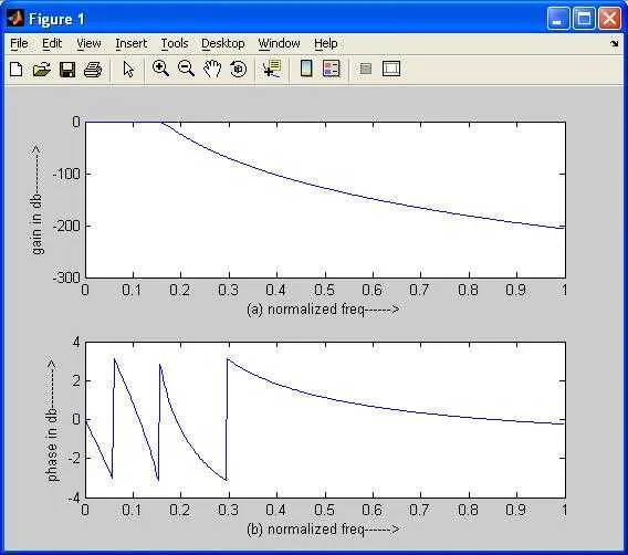
The code above implements a Butterworth Low-Pass filter. It takes passband ripple (rp), stopband ripple (rs), passband frequency (wp), stopband frequency (ws), and sampling frequency (fs) as inputs. The buttord function determines the filter order (n) and cutoff frequency (wn). The butter function then calculates the filter coefficients (b and a). Finally, the frequency response is computed and plotted.
Here’s an example of the output plot:
Butterworth High-Pass Filter MATLAB Code
%Butterworth High Pass Filter
clc;
close all;
clear all;
format long;
rp=input('enter the passband ripple:(default:0.2)');
rs=input('enter the stopband ripple:(default:40)');
wp=input('enter the passband frequency:(default:2000)');
ws=input('enter the stopband frequency:(default:3500)');
fs=input('enter the sampling frequency:(default:8000)');
w1=2*wp/fs;
w2=2*ws/fs;
[n,wn]=buttord(w1,w2,rp,rs,'s');
[z,p,k]= butter(n,wn);
[b,a]=butter(n,wn,'high','s');
w=0:0.01:pi;
[h,om]=freqs(b,a,w);
m=20*log10(abs(h));
an=angle(h);
subplot(2,1,1);
plot(om/pi,m);
ylabel('gain in db--------->');
xlabel('(a) normalized freq------>');
subplot(2,1,2);
plot(om/pi,an);
ylabel('phase in db--------->');
xlabel('(b) normalized freq------>');
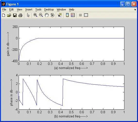
The code above implements a Butterworth High-Pass filter. The structure is similar to the low-pass filter, but the butter function is called with the 'high' argument to specify a high-pass filter design.
Here’s an example of the output plot:
Continue Learning Filter Fundamentals & Terminology
- Lumped Element Filter : Key Advantages & Disadvantages
- Microstrip Based RF Low Pass Filter Design Example
- Understanding Filter Terms
- RF Filters : Types, Selection Guide, Advantages & Disadvantages
- Active vs Passive Filters
- Analog vs Digital Filters
- Butterworth, Chebyshev, Bessel, and Elliptic Filters
- FIR Filter vs IIR Filter
- Understanding CIC (Cascaded Integrator-Comb) Filters
- Pi Filter: Advantages & Disadvantages
- Active vs Passive Harmonic Filters
Explore More RF, Microwave & High Frequency Filters
- SAW vs BAW Filters
- FBAR Filters: Advantages and Disadvantages
- Cavity Filter Types: Advantages & Disadvantages
- Microstrip Filter Structures: Basics and Types
- LTCC Filter Types
- MMIC RF Reflectionless Filter
- Suspended Substrate Stripline Filter
Explore MATLAB Signal Processing & Filtering
- Analog Filter Implementation in MATLAB
- FIR Digital Filter (MATLAB Source Code)
- Low Pass FIR Filter Implementation in MATLAB
- FIR Digital Filter Design: Kaiser Window in MATLAB
- FIR Digital Filter: Rectangular Window in MATLAB
- FIR Digital Filter: Triangular Window in MATLAB
- Low Pass IIR Butterworth Digital Filter (MATLAB Code)
- Butterworth Filter Design in MATLAB
- Convolution (MATLAB Source Code)
- Auto/Cross-Correlation in MATLAB
- 16-point FFT/DFT MATLAB Code using Decimation in Frequency
- IFFT MATLAB: Inverse Fast Fourier Transform
- Decimation/Downsampling (MATLAB Source Code)
- MATLAB Code for Interpolation and Up-Sampling
- Plotting 2D/3D Curves in MATLAB