
MSK Modulation in MATLAB: Code, Explanation, and Results
Advertisement
This document provides a comprehensive guide to Minimum Shift Keying (MSK) modulation using MATLAB. It includes the MATLAB source code, explanations of the code’s functionality, and the expected input and output.
Introduction to MSK Modulation
MSK modulation is a type of continuous-phase frequency-shift keying (CPFSK). It’s closely related to Offset Quadrature Phase-Shift Keying (OQPSK).
- OQPSK limitation: OQPSK can have a maximum phase shift of 90 degrees between transitions (45 degree for each I and Q channel).
- MSK advantage: MSK ensures a 0-degree phase shift between transitions, creating a smoother signal.
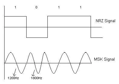
- Wave Shaping: Instead of rectangular pulses like in OQPSK, MSK uses half-cycle sine waves to shape the signal.
- Frequency Difference: The frequencies representing logic ‘0’ and logic ‘1’ in MSK differ by half the data rate.
Mathematical Representation of MSK
The following image depicts the MSK equation:

And this image shows the MSK waveform:
For a more detailed comparison, you can refer to MSK versus GMSK, which explains the time-domain waveforms and mathematical equations of both MSK and GMSK modulation.
MATLAB Code for MSK Modulation
Here’s the MATLAB code for MSK modulation:
clear;
clc;

b = input('Enter the Bit stream \n ');
% b = [0 1 0 1 1 1 0]; % Example bitstream
n = length(b);
t = 0:.01:n;
x = 1:1:(n+2)*100;

for i = 1:n
    if (b(i) == 0)
        b_p(i) = -1;
    else
        b_p(i) = 1;
    end
    for j = i:.1:i+1
        bw(x(i*100:(i+1)*100)) = b_p(i);
        if (mod(i,2) == 0)
            bow(x(i*100:(i+1)*100)) = b_p(i);
            bow(x((i+1)*100:(i+2)*100)) = b_p(i);
        else
            bew(x(i*100:(i+1)*100)) = b_p(i);
            bew(x((i+1)*100:(i+2)*100)) = b_p(i);
        end
        if (mod(n,2)~= 0)
            bow(x(n*100:(n+1)*100)) = -1;
            bow(x((n+1)*100:(n+2)*100)) = -1;
        end
    end
end

bw = bw(100:end);
bew = bew(100:(n+1)*100);
bow = bow(200:(n+2)*100);

wot = 2*pi*t*(5/4);
Wt = 2*pi*t/(4*1);

st = bow.*sin(wot+(bew.*bow).*Wt);

subplot(4,1,1)
plot(t,bw)
grid on ;
axis([0 n -2 +2])

subplot(4,1,2)
plot(t,bow)
grid on ;
axis([0 n -2 +2])

subplot(4,1,3)
plot(t,bew)
grid on ;
axis([0 n -2 +2])

subplot(4,1,4)
plot(t,st)
grid on ;
axis([0 n -2 +2])

Fs=5/4;
%figure
%periodogram(st)
S = fft(st,65);
PSS = S.* conj(S) / 65;
f = 1000*(-16:16)/65;
figure
plot(f,PSS(1:33))
Code Explanation
-
Initialization:
clear; clc;: Clears the workspace and command window.b = input('Enter the Bit stream \n ');: Prompts the user to enter the bit stream.n = length(b);: Determines the length of the bit stream.t = 0:.01:n;: Creates a time vector for plotting.x = 1:1:(n+2)*100;: Creates an index vector.
-
Bit Conversion and Wave Shaping:
- The code iterates through the bit stream
b. - If a bit is ‘0’, it’s converted to -1; otherwise, it’s converted to 1.
bw,bew, andboware vectors used for shaping the waveforms. The if/else conditions inside the for loops are responsible for creating the offset in the I and Q channels.bwrepresents the original bit sequence,bewrepresents the even bits, andbowrepresents the odd bits.- These are used to create the half-sine wave shaping and staggering of I and Q components.
- The code iterates through the bit stream
-
MSK Modulation:
wot = 2*pi*t*(5/4);: Calculates the frequency term.Wt = 2*pi*t/(4*1);: Calculates the phase term.st = bow.*sin(wot+(bew.*bow).*Wt);: Generates the MSK modulated signal. This is the core of the MSK modulation. The equation combines the odd and even bit streams (bow and bew), along with the time-varying frequency and phase components, to produce the final MSK waveform.
-
Plotting:
subplot(4,1,...): Creates subplots to display the waveforms ofbw,bow,bew, and the modulated signalst.plot(t, ...): Plots the waveforms.grid on;: Adds grid lines for better readability.axis([0 n -2 +2]);: Sets the axis limits.
-
Power Spectral Density (PSD) Estimation:
Fs=5/4;: Sets the sampling frequency.S = fft(st,65);: Computes the Fast Fourier Transform (FFT) of the modulated signal.PSS = S.* conj(S) / 65;: Calculates the power spectral density.f = 1000*(-16:16)/65;: Creates a frequency vector.figure;: Opens a new figure.plot(f,PSS(1:33));: Plots the PSD.
Input and Output of the MATLAB Code
Input
When you run the MSKModulation.m file, the code prompts you to enter the bit stream:
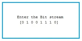
Enter the bit stream as a row vector (e.g., [0 1 0 1 1 1 0]).
Output
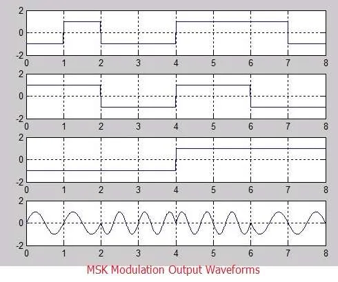
After providing the input and pressing “ENTER”, you will see the following plots:
- Bit Stream (bw): The original binary data stream.
- Odd Bit Stream (bow): The odd-indexed bits with pulse shaping.
- Even Bit Stream (bew): The even-indexed bits with pulse shaping.
- MSK Modulated Signal (st): The final modulated waveform.
- Power Spectral Density (PSD): Frequency domain representation of the modulated signal.
Explore MATLAB Wireless Communications & Modulation
- AM/FM/PM Modulation in MATLAB
- ASK Modulation in MATLAB
- FSK Modulation in MATLAB
- MSK Modulation in MATLAB
- GMSK Modulation in MATLAB
- PSK Modulation (MATLAB Code)
- BPSK, QPSK, 16-QAM, 64-QAM (MATLAB Code)
- On-Off Keying (OOK) (MATLAB Code)
- OFDM (MATLAB Code)
- OFDMA Basics (MATLAB Code)
- SC-FDMA Basics (MATLAB Implementation)
- WiMAX OFDM Basics (MATLAB Code)
- WLAN OFDM Basics (MATLAB Code)
- LTE Basics (MATLAB Code)
- OFCDM (MATLAB Code)
- Beamforming (MATLAB Code QAM)
- 2x2 MIMO & STBC (MATLAB Code)
- CDMA (MATLAB Code)
- Zigbee Transceiver (MATLAB Code)
Continue Learning Modulation Types
- AM Vs. FM Vs. PM : Difference between Analog Modulation Techniques
- ASK Vs. FSK Vs. PSK : Difference between Digital Modulation Techniques
- PAM Vs. PWM Vs. PPM : Difference between Pulse Modulation Techniques
- BPSK Vs. QPSK : Key Differences
- 16-QAM Vs. 64-QAM Vs. 256-QAM : Key Differences
- 512-QAM Vs. 1024-QAM Vs. 2048-QAM Vs. 4096-QAM
- 4096QAM Modulation Used in Wi-Fi 7
- MSK Vs. GMSK : Modulation Technique used in GSM
- LORa Modulation Used in LoRaWAN
- 10% ASK & 100% ASK Modulation used in NFC
- OOK Vs. VPPM Vs. CSK : Visible Light Communication (VLC) Modulation Techniques
- QPSK Vs. OQPSK Vs. PI/4 QPSK
- PAM4 Modulation Used in Gigabit Ethernet
- CCK Vs. DSSS Vs. OFDM Used in WLAN (Wi-Fi) Standards