Decimation in Frequency 16-point FFT/DFT MATLAB Code
Advertisement
This section presents MATLAB source code for Decimation in Frequency FFT or DFT. It validates the code by comparing the FFT output with MATLAB’s built-in FFT function.
This page details a 16-point Decimation in Frequency FFT/DFT with Bit-reversed OUTPUT. While radix-2 FFTs are the most common, other radices (small numbers less than 10) are sometimes used. For example, radix-4 is appealing because the twiddle factors are simply 1, -1, j, or -j, requiring no multiplications.
What is FFT Radix?
Radix refers to the size of an FFT decomposition.
Twiddle Factor
Twiddle factors are the coefficients used to combine results from a previous stage as inputs to the next stage. They are calculated as:
where N = 16 (for a 16-point FFT) and n ranges from 0 to 7.
Decimation in Time FFT
FFTs can be decomposed using DFTs of even and odd points, which is called Decimation in Time FFT.
Decimation in Frequency FFT
FFTs can be decomposed using a first half/second half approach, which is called Decimation in Frequency FFT.
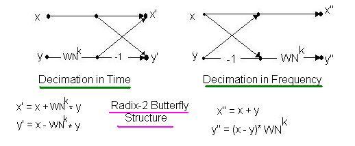
Both Decimation in Time and Decimation in Frequency can be implemented with the same method; only the butterfly structure differs, as shown in the figure.

%16 POINT FFT with Bit %reversed OUTPUT....
%Decimation in Frequency

clear all;
close all;
clc;

%Input Coefficients
x0  = 1 + i*1;
x1  = 2 + i*1;
x2  = 1 - i*2;
x3  = 2 - i*1;
x4  = 2 + i*3;
x5  = 3 + i*2;
x6  = 1 + i*3;
x7  = 3 + i*1;
x8  = -3 + i*3;
x9  =  3 - i*3;
x10 = -1 - i*1;
x11 = -3 - i*3;
x12 = 3 - i*3;
x13 = -1 - i*1;
x14 = -3 - i*3;
x15 = 1 + i*1;
x=[x0 ;x1 ;x2 ;x3 ;x4 ;x5; x6; x7; x8; x9; x10; x11; x12 ;x13; x14 ;x15];

%Twiddle Factors
%3rd stage
tc0=1.0000;
tc1=0.9239 - 0.3827i;
tc2=0.7071 - 0.7071i;
tc3=0.3827 - 0.9239i;
tc4=0.0000 - 1.0000i;
tc5=-0.3827 - 0.9239i;
tc6=-0.7071 - 0.7071i;
tc7=-0.9239 - 0.3827i;

%Twiddle Factors
%2nd stage
tb0=1.0000;
tb1=0.7071 - 0.7071i;
tb2=0.0000 - 1.0000i;
tb3=-0.7071 - 0.7071i;

%1st stage
ta0=1.0000;
ta1=0.0000 - 1.0000i;

%%Stage 3 outputs
s3_0    =   x0 + x8;
s3_1    =   x1 + x9;
s3_2    =   x2 + x10;
s3_3    =   x3 + x11;
s3_4    =   x4 + x12;
s3_5    =   x5 + x13;
s3_6    =   x6 + x14;
s3_7    =   x7 + x15;
s3_8    =   (x0 - x8)*tc0;
s3_9    =   (x1 - x9)*tc1;
s3_10   =   (x2 - x10)*tc2;
s3_11   =   (x3 - x11)*tc3;
s3_12   =   (x4 - x12)*tc4;
s3_13   =   (x5 - x13)*tc5;
s3_14   =   (x6 - x14)*tc6;
s3_15   =   (x7 - x15)*tc7;

Stage3 =[s3_0;s3_1;s3_2;s3_3;s3_4; s3_5;s3_6;s3_7;s3_8;s3_9; s3_10;s3_11;s3_12; s3_13;s3_14;s3_15];

%%Stage 2 outputs
s2_0    =   s3_0 + s3_4;
s2_1    =   s3_1 + s3_5;
s2_2    =   s3_2 + s3_6;
s2_3    =   s3_3 + s3_7;
s2_4    =   (s3_0 - s3_4)*tb0;
s2_5    =   (s3_1 - s3_5)*tb1;
s2_6    =   (s3_2 - s3_6)*tb2;
s2_7    =   (s3_3 - s3_7)*tb3;
s2_8    =    s3_8 + s3_12;
s2_9    =    s3_9 + s3_13;
s2_10    =   s3_10 + s3_14;
s2_11    =   s3_11 + s3_15;
s2_12    =   (s3_8 - s3_12)*tb0;
s2_13    =   (s3_9 - s3_13)*tb1;
s2_14    =   (s3_10 - s3_14)*tb2;
s2_15    =   (s3_11 - s3_15)*tb3;

Stage2 =[s2_0;s2_1;s2_2;s2_3;s2_4; s2_5;s2_6;s2_7;s2_8;s2_9; s2_10;s2_11;s2_12; s2_13;s2_14;s2_15];

%%stage 1
s1_0    =     s2_0    +   s2_2;
s1_1    =     s2_1    +   s2_3;
s1_2    =    (s2_0    -   s2_2) * ta0;
s1_3    =    (s2_1    -   s2_3) * ta1;
s1_4    =     s2_4    +   s2_6;
s1_5    =     s2_5    +   s2_7;
s1_6    =    (s2_4    -   s2_6) * ta0;
s1_7    =    (s2_5    -   s2_7) * ta1;
s1_8    =     s2_8    +   s2_10;
s1_9    =     s2_9    +   s2_11;
s1_10    =   (s2_8    -   s2_10) * ta0;
s1_11    =   (s2_9    -   s2_11) * ta1;
s1_12    =    s2_12    +   s2_14;
s1_13    =    s2_13    +   s2_15;
s1_14    =   (s2_12    -   s2_14) * ta0;
s1_15    =   (s2_13    -   s2_15) * ta1;

%%stage 0
s0_0    =   s1_0    +  s1_1;
s0_1    =   s1_0    -  s1_1;
s0_2    =   s1_2    +  s1_3;
s0_3    =   s1_2    -  s1_3;
s0_4    =   s1_4    +  s1_5;
s0_5    =   s1_4    -  s1_5;
s0_6    =   s1_6    +  s1_7;
s0_7    =   s1_6    -  s1_7;
s0_8    =   s1_8    +  s1_9;
s0_9    =   s1_8    -  s1_9;
s0_10    =  s1_10    +  s1_11;
s0_11    =  s1_10    -  s1_11;
s0_12    =  s1_12    +  s1_13;
s0_13    =  s1_12    -  s1_13;
s0_14    =  s1_14    +  s1_15;
s0_15    =  s1_14    -  s1_15;

Y = [s0_0;s0_1;s0_2;s0_3;s0_4; s0_5;s0_6;s0_7;s0_8;s0_9; s0_10;s0_11;s0_12;s0_13; s0_14;s0_15];

% i=0:15;
% de2bi(i);
% D=bi2de(ans,'left-msb');
% D1=D+1;
Y=[Y(1);Y(9);Y(5);Y(13);Y(3); Y(11);Y(7);Y(15);Y(2); Y(10);Y(6);Y(14); Y(4);Y(12);Y(8);Y(16)];

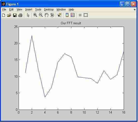
figure;plot(abs(Y));
title('Our FFT result');

%plotting my FFT
%MATLAB built-in FFT MATLAB function
Y_fft = fft(x,16);
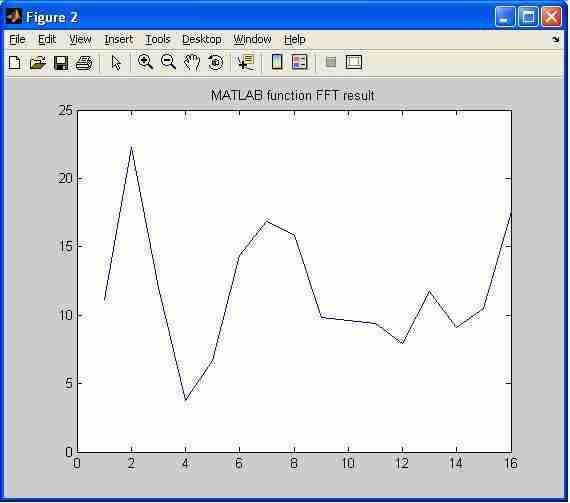
figure; plot(abs(Y_fft));
title('MATLAB function FFT result');
%plotting matlab's built in FFT
16-point FFT MATLAB Output

16-point FFT MATLAB Function Output

Advertisement
 RF
RF


